二次代价函数的问题

当使用二次代价函数的时候，

$C=\frac{(y-a)^2}{2}$

其中$a$时神经元的输出，$a=\sigma(z)$，其中$z=wx+b$。这时计算偏导数

$\frac{\partial C}{\partial w}= (a-y)\sigma'(z)x$

$\frac{\partial C}{\partial b}=(a-y)\sigma'(z)$

我们来看一下$sigmoid$函数的图形

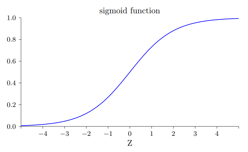
从图中可以看出，当神经元的输出接近于1的时候，曲线变得相当平，所以$\sigma'(z)$就很小，于是$\frac{\partial C}{\partial w}$和$\frac{\partial C}{\partial b}$也会很小，这个会导致在梯度下降过程中学习变得缓慢。

引入交叉熵代价函数

定义交叉熵代价函数：

$C= -\frac{1}{n}\displaystyle\sum_{x}[y\mathrm{ln}a+(1-y)\mathrm{ln}(1-a))]$

交叉熵有一个比代价函数更好的特性就是它避免了学习速度下降的问题。
我们来计算交叉熵函数的偏导数，将$a = \sigma(z)$ 代入上式，并求偏导数

$\frac{\partial C}{\partial w_j}= -\frac{1}{n}\displaystyle\sum_{x}\big(\frac{y}{\sigma(z)}-\frac{1-y}{1-\sigma(z)}\big)\frac{\partial \sigma(z)}{\partial w_j}$

$=-\frac{1}{n}\displaystyle\sum_{x}\big(\frac{y}{\sigma(z)}-\frac{1-y}{1-\sigma(z)}\big)\sigma'(z)x_j$

$=-\frac{1}{n}\displaystyle\sum_{x}\frac{\sigma(z)-y}{\sigma(z)(1-\sigma(z))}\sigma'(z)x_j$

其中$\sigma(z)=\frac{1}{1+e^{-x}}$，计算可得$\sigma'(z)=\sigma(z)(1-\sigma(z))$，于是得到

$\frac{\partial C}{\partial w_j}=-\frac{1}{n}\displaystyle\sum_{x}(\sigma(z)-y)x_j$

这里权重的学习速度受到$\sigma(z)-y$的影响，也就是输出中的误差的控制。更大的误差会有更大的学习速度。

同样的，我们可以得到关于偏置的偏导数

$\frac{\partial C}{\partial b}=-\frac{1}{n}\displaystyle\sum_{x}(\sigma(z)-y)$

交叉熵函数扩展到多神经元的多层神经网络上

假设$y=y1,y2,...$是输出神经元上的目标值，而$a^L_1,a^L_2,...$时实际的输出值，那么我们定义交叉熵如下

$C= -\frac{1}{n}\displaystyle\sum_{x}\displaystyle\sum_{y}[y_j\mathrm{ln}a^L_j+(1-y_j)\mathrm{ln}(1-a^L_j))]$

那么我们应该在什么时候用交叉熵来替换二次代价函数？

实际上，如果输出神经元是S型时，交叉熵函数一般都是更好的选择。为什么？考虑一下我们初始化网络的权重和偏置时，通常使用某种随机方法。可能会发生这样的情况，这些初始选择会对某些训练输入的误差相当明显，比如说，目标输出是1，而实际值是0，或者完全反过来。如果使用二次代价函数，那么就会导致学习速度下降。

改进交叉熵函数代码

class QuadraticCost(object):

    @staticmethod
    def fn(a, y):
        """Return the cost associated with an output ``a`` and desired output
        ``y``.

        """
        return 0.5*np.linalg.norm(a-y)**2

    @staticmethod
    def delta(z, a, y):
        """Return the error delta from the output layer."""
        return (a-y) * sigmoid_prime(z)


class CrossEntropyCost(object):

    @staticmethod
    def fn(a, y):
        """Return the cost associated with an output ``a`` and desired output
        ``y``.  Note that np.nan_to_num is used to ensure numerical
        stability.  In particular, if both ``a`` and ``y`` have a 1.0
        in the same slot, then the expression (1-y)*np.log(1-a)
        returns nan.  The np.nan_to_num ensures that that is converted
        to the correct value (0.0).

        """
        return np.sum(np.nan_to_num(-y*np.log(a)-(1-y)*np.log(1-a)))

    @staticmethod
    def delta(z, a, y):
        """Return the error delta from the output layer.  Note that the
        parameter ``z`` is not used by the method.  It is included in
        the method's parameters in order to make the interface
        consistent with the delta method for other cost classes.

        """
        return (a-y)

其中 QuadraticCost 是二次代价函数，CrossEntropyCost 是交叉熵代价函数。